6.3. YODA-compliant data analysis projects

Now that you know about the YODA principles, it is time to start working on DataLad-101’s midterm project. Because the midterm project guidelines require a YODA-compliant data analysis project, you will not only have theoretical knowledge about the YODA principles, but also gain practical experience.

In principle, you can prepare YODA-compliant data analyses in any programming language of your choice. But because you are already familiar with the Python programming language, you decide to script your analysis in Python. Delighted, you find out that there is even a Python API for DataLad’s functionality that you can read about in a Findoutmore on DataLad in Python.

DataLad’s Python API

Whatever you can do with DataLad from the command line, you can also do it with DataLad’s Python API. Thus, DataLad’s functionality can also be used within interactive Python sessions or Python scripts. All of DataLad’s user-oriented commands are exposed via datalad.api. Thus, any command can be imported as a stand-alone command like this:

>>> from datalad.api import <COMMAND>

Alternatively, to import all commands, one can use

>>> import datalad.api as dl

and subsequently access commands as dl.get(), dl.clone(), and so forth.

The developer documentation of DataLad lists an overview of all commands, but naming is congruent to the command line interface. The only functionality that is not available at the command line is datalad.api.Dataset, DataLad’s core Python data type. Just like any other command, it can be imported like this:

>>> from datalad.api import Dataset

or like this:

>>> import datalad.api as dl
>>> dl.Dataset()

A Dataset is a class that represents a DataLad dataset. In addition to the stand-alone commands, all of DataLad’s functionality is also available via methods of this class. Thus, these are two equally valid ways to create a new dataset with DataLad in Python:

>>> from datalad.api import create, Dataset
# create as a stand-alone command
>>> create(path='scratch/test')
[INFO   ] Creating a new annex repo at /.../scratch/test
Out[3]: <Dataset path=/home/me/scratch/test>
# create as a dataset method
>>> ds = Dataset(path='scratch/test')
>>> ds.create()
[INFO   ] Creating a new annex repo at /.../scratch/test
Out[3]: <Dataset path=/home/me/scratch/test>

As shown above, the only required parameter for a Dataset is the path to its location, and this location may or may not exist yet.

Stand-alone functions have a dataset= argument, corresponding to the -d/--dataset option in their command-line equivalent. You can specify the dataset= argument with a path (string) to your dataset (such as dataset='.' for the current directory, or dataset='path/to/ds' to another location). Alternatively, you can pass a Dataset instance to it:

>>> from datalad.api import save, Dataset
# use save with dataset specified as a path
>>> save(dataset='path/to/dataset/')
# use save with dataset specified as a dataset instance
>>> ds = Dataset('path/to/dataset')
>>> save(dataset=ds, message="saving all modifications")
# use save as a dataset method (no dataset argument)
>>> ds.save(message="saving all modifications")

Use cases for DataLad’s Python API

Using the command line or the Python API of DataLad are both valid ways to accomplish the same results. Depending on your workflows, using the Python API can help to automate dataset operations, provides an alternative to the command line, or could be useful for scripting reproducible data analyses. One unique advantage of the Python API is the Dataset: As the Python API does not suffer from the startup time cost of the command line, there is the potential for substantial speed-up when doing many calls to the API, and using a persistent Dataset object instance. You will also notice that the output of Python commands can be more verbose as the result records returned by each command do not get filtered by command-specific result renderers. Thus, the outcome of dl.status('myfile') matches that of datalad status (manual) only when -f/--output-format is set to json or json_pp, as illustrated below.

>>> import datalad.api as dl
>>> dl.status('myfile')
[{'type': 'file',
'gitshasum': '915983d6576b56792b4647bf0d9fa04d83ce948d',
'bytesize': 85,
'prev_gitshasum': '915983d6576b56792b4647bf0d9fa04d83ce948d',
'state': 'clean',
'path': '/home/me/my-ds/myfile',
'parentds': '/home/me/my-ds',
'status': 'ok',
'refds': '/home/me/my-ds',
'action': 'status'}]

$ datalad -f json_pp status myfile
 {"action": "status",
  "bytesize": 85,
  "gitshasum": "915983d6576b56792b4647bf0d9fa04d83ce948d",
  "parentds": "/home/me/my-ds",
  "path": "/home/me/my-ds/myfile",
  "prev_gitshasum": "915983d6576b56792b4647bf0d9fa04d83ce948d",
  "refds": "/home/me/my-ds/",
  "state": "clean",
  "status": "ok",
  "type": "file"}

Use DataLad in languages other than Python

While there is a dedicated API for Python, DataLad’s functions can of course also be used with other programming languages, such as Matlab, or R, via standard system calls.

Even if you do not know or like Python, you can just copy-paste the code and follow along – the high-level YODA principles demonstrated in this section generalize across programming languages.

For your midterm project submission, you decide to create a data analysis on the iris flower data set. It is a multivariate dataset on 50 samples of each of three species of Iris flowers (Setosa, Versicolor, or Virginica), with four variables: the length and width of the sepals and petals of the flowers in centimeters. It is often used in introductory data science courses for statistical classification techniques in machine learning, and widely available – a perfect dataset for your midterm project!

Turn data analysis into dynamically generated documents

Beyond the contents of this section, we have transformed the example analysis also into a template to write a reproducible paper. If you are interested in checking that out, please head over to github.com/datalad-handbook/repro-paper-sketch/.

6.3.1. Raw data as a modular, independent entity

The first YODA principle stressed the importance of modularity in a data analysis project: Every component that could be used in more than one context should be an independent component.

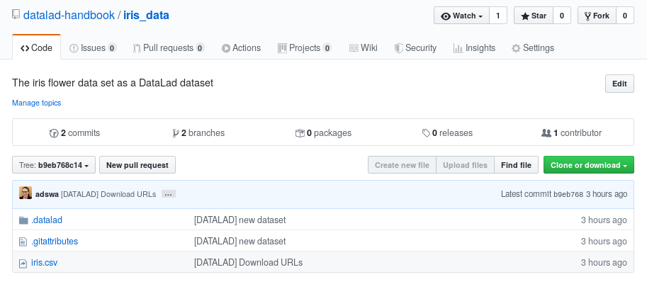
The first aspect this applies to is the input data of your dataset: There can be thousands of ways to analyze it, and it is therefore immensely helpful to have a pristine raw iris dataset that does not get modified, but serves as input for these analysis. As such, the iris data should become a standalone DataLad dataset. For the purpose of this analysis, the DataLad handbook provides an iris_data dataset at https://github.com/datalad-handbook/iris_data.

You can either use this provided input dataset, or find out how to create an independent dataset from scratch in a dedicated Findoutmore.

Creating an independent input dataset

If you acquire your own data for a data analysis, you will have to turn it into a DataLad dataset in order to install it as a subdataset. Any directory with data that exists on your computer can be turned into a dataset with datalad create --force (manual) and a subsequent datalad save -m "add data" . (manual) to first create a dataset inside of an existing, non-empty directory, and subsequently save all of its contents into the history of the newly created dataset.

To create the iris_data dataset at https://github.com/datalad-handbook/iris_data we first created a DataLad dataset…

$ # make sure to move outside of DataLad-101!
$ cd ../
$ datalad create iris_data
create(ok): /home/me/dl-101/iris_data (dataset)

and subsequently got the data from a publicly available GitHub Gist, a code snippet, or other short standalone information with a datalad download-url (manual) command:

$ cd iris_data
$ datalad download-url https://gist.githubusercontent.com/netj/8836201/raw/6f9306ad21398ea43cba4f7d537619d0e07d5ae3/iris.csv
download_url(ok): /home/me/dl-101/iris_data/iris.csv (file)
add(ok): iris.csv (file)
save(ok): . (dataset)

Finally, we published the dataset to GitHub.

With this setup, the iris dataset (a single comma-separated (.csv) file) is downloaded, and, importantly, the dataset recorded where it was obtained from thanks to datalad download-url, thus complying to the second YODA principle. This way, upon installation of the dataset, DataLad knows where to obtain the file content from. You can datalad clone (manual) the iris dataset and find out with a git annex whereis iris.csv command.

“Nice, with this input dataset I have sufficient provenance capture for my input dataset, and I can install it as a modular component”, you think as you mentally tick off YODA principle number 1 and 2. “But before I can install it, I need an analysis superdataset first.”

6.3.2. Building an analysis dataset

There is an independent raw dataset as input data, but there is no place for your analysis to live, yet. Therefore, you start your midterm project by creating an analysis dataset. As this project is part of DataLad-101, you do it as a subdataset of DataLad-101. Remember to specify the --dataset option of datalad create to link it as a subdataset!

You naturally want your dataset to follow the YODA principles, and, as a start, you use the cfg_yoda procedure to help you structure the dataset[1]:

$ # inside of DataLad-101
$ datalad create -c yoda --dataset . midterm_project
[INFO] Running procedure cfg_yoda
[INFO] == Command start (output follows) =====
[INFO] == Command exit (modification check follows) =====
run(ok): /home/me/dl-101/DataLad-101/midterm_project (dataset) [VIRTUALENV/bin/python /home/a...]
add(ok): midterm_project (dataset)
add(ok): .gitmodules (file)
save(ok): . (dataset)
create(ok): midterm_project (dataset)

The datalad subdatasets (manual) command can report on which subdatasets exist for DataLad-101. This helps you verify that the command succeeded and the dataset was indeed linked as a subdataset to DataLad-101:

$ datalad subdatasets
subdataset(ok): midterm_project (dataset)
subdataset(ok): recordings/longnow (dataset)

Not only the longnow subdataset, but also the newly created midterm_project subdataset are displayed – wonderful!

But back to the midterm project now. So far, you have created a pre-structured analysis dataset. As a next step, you take care of installing and linking the raw dataset for your analysis adequately to your midterm_project dataset by installing it as a subdataset. Make sure to install it as a subdataset of midterm_project, and not DataLad-101!

$ cd midterm_project
$ # we are in midterm_project, thus -d . points to the root of it.
$ datalad clone -d . \
  https://github.com/datalad-handbook/iris_data.git \
  input/
[INFO] Remote origin not usable by git-annex; setting annex-ignore
install(ok): input (dataset)
add(ok): input (dataset)
add(ok): .gitmodules (file)
save(ok): . (dataset)
add(ok): .gitmodules (file)
save(ok): . (dataset)

Note that we did not keep its original name, iris_data, but rather provided a path with a new name, input, because this much more intuitively comprehensible.

After the input dataset is installed, the directory structure of DataLad-101 looks like this:

$ cd ../
$ tree -d
$ cd midterm_project
.
├── books
├── code
├── midterm_project
│   ├── code
│   └── input
└── recordings
    └── longnow
        ├── Long_Now__Conversations_at_The_Interval
        └── Long_Now__Seminars_About_Long_term_Thinking

9 directories

Importantly, all of the subdatasets are linked to the higher-level datasets, and despite being inside of DataLad-101, your midterm_project is an independent dataset, as is its input/ subdataset. An overview is shown in Fig. 6.4.

Fig. 6.4 Overview of (linked) datasets in DataLad-101.

6.3.3. YODA-compliant analysis scripts

Now that you have an input/ directory with data, and a code/ directory (created by the YODA procedure) for your scripts, it is time to work on the script for your analysis. Within midterm_project, the code/ directory is where you want to place your scripts.

But first, you plan your research question. You decide to do a classification analysis with a k-nearest neighbors algorithm[2]. The iris dataset works well for such questions. Based on the features of the flowers (sepal and petal width and length) you will try to predict what type of flower (Setosa, Versicolor, or Virginica) a particular flower in the dataset is. You settle on two objectives for your analysis:

1. Explore and plot the relationship between variables in the dataset and save the resulting graphic as a first result.

2. Perform a k-nearest neighbor classification on a subset of the dataset to predict class membership (flower type) of samples in a left-out test set. Your final result should be a statistical summary of this prediction.

To compute the analysis you create the following Python script inside of code/:

$ cat << EOT > code/script.py

import argparse
import pandas as pd
import seaborn as sns
from sklearn import model_selection
from sklearn.neighbors import KNeighborsClassifier
from sklearn.metrics import classification_report

parser = argparse.ArgumentParser(description="Analyze iris data")
parser.add_argument('data', help="Input data (CSV) to process")
parser.add_argument('output_figure', help="Output figure path")
parser.add_argument('output_report', help="Output report path")
args = parser.parse_args()

# prepare the data as a pandas dataframe
df = pd.read_csv(args.data)
attributes = ["sepal_length", "sepal_width", "petal_length","petal_width", "class"]
df.columns = attributes

# create a pairplot to plot pairwise relationships in the dataset
plot = sns.pairplot(df, hue='class', palette='muted')
plot.savefig(args.output_figure)

# perform a K-nearest-neighbours classification with scikit-learn
# Step 1: split data in test and training dataset (20:80)
array = df.values
X = array[:,0:4]
Y = array[:,4]
test_size = 0.20
seed = 7
X_train, X_test, Y_train, Y_test = model_selection.train_test_split(
    X, Y,
    test_size=test_size,
    random_state=seed)
# Step 2: Fit the model and make predictions on the test dataset
knn = KNeighborsClassifier()
knn.fit(X_train, Y_train)
predictions = knn.predict(X_test)

# Step 3: Save the classification report
report = classification_report(Y_test, predictions, output_dict=True)
df_report = pd.DataFrame(report).transpose().to_csv(args.output_report)

EOT

This script will

• take three positional arguments: The input data, a path to save a figure under, and path to save the final prediction report under. By including these input and output specifications in a datalad run (manual) command when we run the analysis, we can ensure that input data is retrieved prior to the script execution, and that as much actionable provenance as possible is recorded[5].

• read in the data, perform the analysis, and save the resulting figure and .csv prediction report into the root of midterm_project/. Note how this helps to fulfil YODA principle 1 on modularity: Results are stored outside of the pristine input subdataset.

A short help text explains how the script shall be used:

$ python code/script.py -h
usage: script.py [-h] data output_figure output_report

Analyze iris data

positional arguments:
   data           Input data (CSV) to process
   output_figure  Output figure path
   output_report  Output report path

optional arguments:
-h, --help     show this help message and exit

The script execution would thus be python3 code/script.py <path-to-input> <path-to-figure-output> <path-to-report-output>. When parametrizing the input and output path parameters, we just need make sure that all paths are relative, such that the midterm_project analysis is completely self-contained within the dataset, contributing to fulfill the second YODA principle.

Let’s run a quick datalad status…

$ datalad status
untracked: code/script.py (file)

… and save the script to the subdataset’s history. As the script completes your analysis setup, we tag the state of the dataset to refer to it easily at a later point with the --version-tag option of datalad save.

$ datalad save -m "add script for kNN classification and plotting" \
  --version-tag ready4analysis \
  code/script.py
add(ok): code/script.py (file)
save(ok): . (dataset)

What is a tag?

tags are markers that you can attach to commits in your dataset history. They can have any name, and can help you and others to identify certain commits or dataset states in the history of a dataset. Let’s take a look at how the tag you just created looks like in your history with git show (manual). Note how we can use a tag just as easily as a commit shasum:

$ git show ready4analysis
commit ca0c7477✂SHA1
Author: Elena Piscopia <elena@example.net>
Date:   Tue Jun 18 16:13:00 2019 +0000

    add script for kNN classification and plotting

diff --git a/code/script.py b/code/script.py
new file mode 100644
index 0000000..c7a6ea9
--- /dev/null
+++ b/code/script.py
@@ -0,0 +1,43 @@

This tag thus identifies the version state of the dataset in which this script was added. Later we can use this tag to identify the point in time at which the analysis setup was ready – much more intuitive than a 40-character shasum! This is handy in the context of a datalad rerun (manual), for example:

$ datalad rerun --since ready4analysis

would rerun any datalad run command in the history performed between tagging and the current dataset state.

Finally, with your directory structure being modular and intuitive, the input data installed, the script ready, and the dataset status clean, you can wrap the execution of the script in a datalad run command. Note that simply executing the script would work as well – thanks to DataLad’s Python API. But using datalad run will capture full provenance, and will make re-execution with datalad rerun easy.

Additional software requirements: pandas, seaborn, sklearn

Note that you need to have the following Python packages installed to run the analysis[3]:

• pandas

• seaborn

• sklearn

The packages can be installed via pip. However, if you do not want to install any Python packages, do not execute the remaining code examples in this section – an upcoming section on datalad containers-run will allow you to perform the analysis without changing your Python software-setup.

You may need to use ‘python’, not ‘python3’

If executing the code below returns an exit code of 9009, there may be no python3 – instead, it is called solely python. Please run the following instead (adjusted for line breaks, you should be able to copy-paste this as a whole):

> datalad run -m "analyze iris data with classification analysis" ^
 --input "input/iris.csv" ^
 --output "pairwise_relationships.png" ^
 --output "prediction_report.csv" ^
 "python code/script.py {inputs} {outputs}"

$ datalad run -m "analyze iris data with classification analysis" \
  --input "input/iris.csv" \
  --output "pairwise_relationships.png" \
  --output "prediction_report.csv" \
  "python3 code/script.py {inputs} {outputs}"
get(ok): input/iris.csv (file) [from web...]
[INFO] == Command start (output follows) =====
[INFO] == Command exit (modification check follows) =====
run(ok): /home/me/dl-101/DataLad-101/midterm_project (dataset) [python3 code/script.py input/iris.csv pa...]
add(ok): pairwise_relationships.png (file)
add(ok): prediction_report.csv (file)
save(ok): . (dataset)

As the successful command summary indicates, your analysis seems to work! Two files were created and saved to the dataset: pairwise_relationships.png and prediction_report.csv. If you want, take a look and interpret your analysis. But what excites you even more than a successful data science project on first try is that you achieved complete provenance capture:

• Every single file in this dataset is associated with an author and a time stamp for each modification thanks to datalad save.

• The raw dataset knows where the data came from thanks to datalad clone and datalad download-url.

• The subdataset is linked to the superdataset thanks to datalad clone -d.

• The datalad run command took care of linking the outputs of your analysis with the script and the input data it was generated from, fulfilling the third YODA principle.

Let’s take a look at the history of the midterm_project analysis dataset:

$ git log --oneline
9aadac7 [DATALAD RUNCMD] analyze iris data with classification analysis
ca0c747 add script for kNN classification and plotting
4f945ed [DATALAD] Added subdataset
18f4a98 Apply YODA dataset setup
bf231d5 [DATALAD] new dataset

“Wow, this is so clean and intuitive!” you congratulate yourself. “And I think this was and will be the fastest I have ever completed a midterm project!” But what is still missing is a human readable description of your dataset. The YODA procedure kindly placed a README.md file into the root of your dataset that you can use for this[4].

$ # with the >| redirection we are replacing existing contents in the file
$ cat << EOT >| README.md

# Midterm YODA Data Analysis Project

## Dataset structure

- All inputs (i.e. building blocks from other sources) are located in input/.
- All custom code is located in code/.
- All results (i.e., generated files) are located in the root of the dataset:
  - "prediction_report.csv" contains the main classification metrics.
  - "output/pairwise_relationships.png" is a plot of the relations between features.

EOT

$ datalad status
 modified: README.md (file)

$ datalad save -m "Provide project description" README.md
add(ok): README.md (file)
save(ok): . (dataset)

Note that one feature of the YODA procedure was that it configured certain files (for example, everything inside of code/, and the README.md file in the root of the dataset) to be saved in Git instead of git-annex. This was the reason why the README.md in the root of the dataset was easily modifiable.

Saving contents with Git regardless of configuration with –to-git

The yoda procedure in midterm_project applied a different configuration within .gitattributes than the text2git procedure did in DataLad-101. Within DataLad-101, any text file is automatically stored in Git. This is not true in midterm_project: Only the existing README.md files and anything within code/ are stored – everything else will be annexed. That means that if you create any other file, even text files, inside of midterm_project (but not in code/), it will be managed by git-annex and content-locked after a datalad save – an inconvenience if it would be a file that is small enough to be handled by Git.

Luckily, there is a handy shortcut to saving files in Git that does not require you to edit configurations in .gitattributes: The --to-git option for datalad save.

$ datalad save -m "add sometextfile.txt" --to-git sometextfile.txt

After adding this short description to your README.md, your dataset now also contains sufficient human-readable information to ensure that others can understand everything you did easily. The only thing left to do is to hand in your assignment. According to the syllabus, this should be done via GitHub.

What is GitHub?

GitHub is a web based hosting service for Git repositories. Among many different other useful perks it adds features that allow collaboration on Git repositories. GitLab is a similar service with highly similar features, but its source code is free and open, whereas GitHub is a subsidiary of Microsoft.

Web-hosting services like GitHub and GitLab integrate wonderfully with DataLad. They are especially useful for making your dataset publicly available, if you have figured out storage for your large files otherwise (as large content cannot be hosted for free by GitHub). You can make DataLad publish large file content to one location and afterwards automatically push an update to GitHub, such that users can install directly from GitHub/GitLab and seemingly also obtain large file content from GitHub. GitHub can also resolve subdataset links to other GitHub repositories, which lets you navigate through nested datasets in the web-interface.

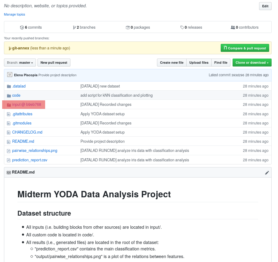
The above screenshot shows the linkage between the analysis project you will create and its subdataset. Clicking on the subdataset (highlighted) will take you to the iris dataset the handbook provides, shown below.

6.3.4. Publishing the dataset to GitHub

For this, you need to

• create a GitHub account, if you do not yet have one

• create a repository for this dataset on GitHub,

• configure this GitHub repository to be a sibling of the midterm_project dataset,

• and publish your dataset to GitHub.

Luckily, DataLad can make this very easy with the datalad create-sibling-github (manual) command (or, for GitLab, datalad create-sibling-gitlab (manual)).

The two commands have different arguments and options. Here, we look at datalad create-sibling-github. The command takes a repository name and GitHub authentication credentials (either in the command line call with options github-login <TOKEN>, with an oauth token stored in the Git configuration, or interactively).

Generate a GitHub token

GitHub deprecated user-password authentication and instead supports authentication via personal access token. To ensure successful authentication, don’t supply your password, but create a personal access token at github.com/settings/tokens[6] instead, and either

• supply the token with the argument --github-login <TOKEN> from the command line,

• or supply the token from the command line when queried for a password

Based on the credentials and the repository name, it will create a new, empty repository on GitHub, and configure this repository as a sibling of the dataset:

Your shell will not display credentials

Don’t be confused if you are prompted for your GitHub credentials, but can’t seem to type – the terminal protects your private information by not displaying what you type. Simply type in what is requested, and press enter.

$ datalad create-sibling-github -d . midtermproject
.: github(-) [https://github.com/adswa/midtermproject.git (git)]
'https://github.com/adswa/midtermproject.git' configured as sibling 'github' for <Dataset path=/home/me/dl-101/DataLad-101/midterm_project>

Verify that this worked by listing the siblings of the dataset:

$ datalad siblings
[WARNING] Failed to determine if github carries annex.
.: here(+) [git]
.: github(-) [https://github.com/adswa/midtermproject.git (git)]

Create-sibling-github internals

Creating a sibling on GitHub will create a new empty repository under the account that you provide and set up a remote to this repository. Upon a datalad push (manual) to this sibling, your datasets history will be pushed there.

On GitHub, you will see a new, empty repository with the name midtermproject. However, the repository does not yet contain any of your dataset’s history or files. This requires publishing the current state of the dataset to this sibling with the datalad push command.

Learn how to push “on the job”

Publishing is one of the remaining big concepts that this handbook tries to convey. However, publishing is a complex concept that encompasses a large proportion of the previous handbook content as a prerequisite. In order to be not too overwhelmingly detailed, the upcoming sections will approach datalad push from a “learning-by-doing” perspective: First, you will see a datalad push to GitHub, and the Findoutmore on the published dataset at the end of this section will already give a practical glimpse into the difference between annexed contents and contents stored in Git when pushed to GitHub. The chapter Third party infrastructure will extend on this, but the section The datalad push command will finally combine and link all the previous contents to give a comprehensive and detailed wrap up of the concept of publishing datasets. In this section, you will also find a detailed overview on how datalad push works and which options are available. If you are impatient or need an overview on publishing, feel free to skip ahead. If you have time to follow along, reading the next sections will get you towards a complete picture of publishing a bit more small-stepped and gently. For now, we will start with learning by doing, and the fundamental basics of datalad push: The command will make the last saved state of your dataset available (i.e., publish it) to the sibling you provide with the --to option.

$ datalad push --to github
copy(ok): pairwise_relationships.png (file) [to github...]
copy(ok): prediction_report.csv (file) [to github...]
publish(ok): . (dataset) [refs/heads/git-annex->github:refs/heads/git-annex ✂FROM✂..✂TO✂]
publish(ok): . (dataset) [refs/heads/main->github:refs/heads/main [new branch]]

Thus, you have now published your dataset’s history to a public place for others to see and clone. Now we will explore how this may look and feel for others.

There is one important detail first, though: By default, your tags will not be published. Thus, the tag ready4analysis is not pushed to GitHub, and currently this version identifier is unavailable to anyone else but you. The reason for this is that tags are viral – they can be removed locally, and old published tags can cause confusion or unwanted changes. In order to publish a tag, an additional git push (manual) with the --tags option is required:

$ git push github --tags

Pushing tags

Note that this is a git push, not datalad push. Tags could be pushed upon a datalad push, though, if one configures (what kind of) tags to be pushed. This would need to be done on a per-sibling basis in .git/config in the remote.*.push configuration. If you had a sibling “github”, the following configuration would push all tags that start with a v upon a datalad push --to github:

$ git config --local remote.github.push 'refs/tags/v*'

This configuration would result in the following entry in .git/config:

[remote "github"]
      url = git@github.com/adswa/midtermproject.git
      fetch = +refs/heads/*:refs/remotes/github/*
      annex-ignore = true
      push = refs/tags/v*

Yay! Consider your midterm project submitted! Others can now install your dataset and check out your data science project – and even better: they can reproduce your data science project easily from scratch (take a look into the Findoutmore to see how)!

On the looks and feels of this published dataset

Now that you have created and published such a YODA-compliant dataset, you are understandably excited how this dataset must look and feel for others. Therefore, you decide to install this dataset into a new location on your computer, just to get a feel for it.

Replace the url in the datalad clone command with the path to your own midtermproject GitHub repository, or clone the “public” midterm_project repository that is available via the Handbook’s GitHub organization at github.com/datalad-handbook/midterm_project:

$ cd ../../
$ datalad clone "https://github.com/adswa/midtermproject.git"
[INFO] Remote origin not usable by git-annex; setting annex-ignore
install(ok): /home/me/dl-101/midtermproject (dataset)

Let’s start with the subdataset, and see whether we can retrieve the input iris.csv file. This should not be a problem, since its origin is recorded:

$ cd midtermproject
$ datalad get input/iris.csv
[INFO] Remote origin not usable by git-annex; setting annex-ignore
install(ok): /home/me/dl-101/midtermproject/input (dataset) [Installed subdataset in order to get /home/me/dl-101/midtermproject/input/iris.csv]
get(ok): input/iris.csv (file) [from web...]

Nice, this worked well. The output files, however, cannot be easily retrieved:

$ datalad get prediction_report.csv pairwise_relationships.png
get(error): pairwise_relationships.png (file) [not available; (Note that these git remotes have annex-ignore set: origin)]
get(error): prediction_report.csv (file) [not available; (Note that these git remotes have annex-ignore set: origin)]

Why is that? This is the first detail of publishing datasets we will dive into. When publishing dataset content to GitHub with datalad push, it is the dataset’s history, i.e., everything that is stored in Git, that is published. The file content of these particular files, though, is managed by git-annex and not stored in Git, and thus only information about the file name and location is known to Git. Because GitHub does not host large data for free, annexed file content always needs to be deposited somewhere else (e.g., a web server) to make it accessible via datalad get (manual). The chapter Third party infrastructure will demonstrate how this can be done. For this dataset, it is not necessary to make the outputs available, though: Because all provenance on their creation was captured, we can simply recompute them with the datalad rerun command. If the tag was published we can simply rerun any datalad run command since this tag:

$ datalad rerun --since ready4analysis

But without the published tag, we can rerun the analysis by specifying its shasum:

$ datalad rerun d715890b✂SHA1
[INFO] run commit d715890; (analyze iris data...)
run.remove(ok): pairwise_relationships.png (file) [Removed file]
run.remove(ok): prediction_report.csv (file) [Removed file]
[INFO] == Command start (output follows) =====
action summary:
  get (notneeded: 2)
[INFO] == Command exit (modification check follows) =====
run(ok): /home/me/dl-101/midtermproject (dataset) [python3 code/script.py]
add(ok): pairwise_relationships.png (file)
add(ok): prediction_report.csv (file)
save(ok): . (dataset)
action summary:
  add (ok: 2)
  get (notneeded: 3)
  run (ok: 1)
  run.remove (ok: 2)
  save (notneeded: 1, ok: 1)

Hooray, your analysis was reproduced! You happily note that rerunning your analysis was incredibly easy – it would not even be necessary to have any knowledge about the analysis at all to reproduce it! With this, you realize again how letting DataLad take care of linking input, output, and code can make your life and others’ lives so much easier. Applying the YODA principles to your data analysis was very beneficial indeed. Proud of your midterm project you cannot wait to use those principles the next time again.

Push internals

The datalad push uses git push, and git annex copy under the hood. Publication targets need to either be configured remote Git repositories, or git-annex special remotes (if they support data upload).

Footnotes

[1]

Note that you could have applied the YODA procedure not only right at creation of the dataset with -c yoda, but also after creation with the datalad run-procedure (manual) command:

$ cd midterm_project
$ datalad run-procedure cfg_yoda

Both ways of applying the YODA procedure will lead to the same outcome.

[2]

The choice of analysis method for the handbook is rather arbitrary, and understanding the k-nearest neighbor algorithm is by no means required for this section.

[3]

It is recommended (but optional) to create a virtual environment and install the required Python packages inside of it:

$ # create and enter a new virtual environment (optional)
$ virtualenv --python=python3 ~/env/handbook
$ . ~/env/handbook/bin/activate

$ # install the Python packages from PyPi via pip
$ pip install seaborn pandas sklearn

[4]

All README.md files the YODA procedure created are version controlled by Git, not git-annex, thanks to the configurations that YODA supplied. This makes it easy to change the README.md file. The previous section detailed how the YODA procedure configured your dataset. If you want to re-read the full chapter on configurations and run-procedures, start with section DIY configurations.

[5]

Alternatively, if you were to use DataLad’s Python API, you could import and expose it as dl.<COMMAND> and dl.get() the relevant files. This however, would not record them as provenance in the dataset’s history.

[6]

Instead of using GitHub’s WebUI you could also obtain a token using the command line GitHub interface (https://github.com/sociomantic-tsunami/git-hub) by running git hub setup (if no 2FA is used).